Validation
validation.RmdValidation
Please note: The validation data are attached with pre-calculated
risk scores and can be loaded with the function
get_validation_data()
To ensure correspondence between values calculated offline and online, a validation data set of 5000 women was generated to cover a wide range of possible combinations:
# Function to generate random samples from a parameter space
sample_parameter_space <- function(parameter_ranges, n_samples = 2500) {
  # parameter_ranges should be a list where each element is either:
  # - a vector of discrete values to sample from
  # - a numeric vector of length 2 specifying [min, max] for continuous variables

  # Initialize result dataframe
  result <- data.frame(matrix(nrow = n_samples, ncol = length(parameter_ranges)))
  names(result) <- names(parameter_ranges)

  # Sample each parameter
  for (param_name in names(parameter_ranges)) {
    param_range <- parameter_ranges[[param_name]]

    if (length(param_range) == 2 && is.numeric(param_range)) {
      # Continuous parameter: sample uniformly between min and max
      result[[param_name]] <- runif(n_samples, min = param_range[1], max = param_range[2])
    } else {
      # Discrete parameter: sample with replacement from provided values
      result[[param_name]] <- sample(param_range, n_samples, replace = TRUE)
    }
  }

  return(result)
}

parameter_ranges <- list(
  # Pregnancy Details
  twins = "no",
  crl1 = NA,
  crl2 = NA,
  crl = 50,
  ga = c(11.3, 14),
  ga_at = "01-01-2024",

  # Maternal Characteristics
  dob = paste0("01-01-", seq(1985, 2006)),
  height = c(150, 190),
  weight = c(40, 180),
  race = c(1, 2, 3, 4, 5),
  smoking = c("yes", "no", "no"),
  mother_pe = c("yes", "no", "no"),
  conception = c(1, 1, 1, 1, 2, 3),

  # Medical History
  chronic_hypertension = c("yes", "no", "no", "no", "no"),
  diabetes_type_i = c("yes", "no", "no", "no", "no"),
  diabetes_type_ii = c("yes", "no", "no", "no", "no"),
  diabetes_drugs = c("diet only", "insulin", "insulin+metformin", "metformin"),
  sle = c("yes", "no", "no", "no", "no", "no", "no", "no", "no", "no"),
  aps = c("yes", "no", "no", "no", "no", "no", "no", "no", "no", "no"),

  # Obstetric History
  previous = "no",
  previous_pe = NA,
  previous_delivered_at = NA,
  previous_ga_weeks     = NA,
  previous_ga_days      = NA,
  previous_interval     = NA,

  # Biophysical Measurements
  map = c(60, 100),
  utpi = c(0.8, 3),
  biophysical_at = "01-01-2024",

  # Biochemical Measurements
  include_plgf = "raw",
  include_pappa = "no",
  plgf_mom = NA,
  plgf = c(10, 80),
  plgf_machine = c("delfia", "kryptor", "roche"),
  pappa_mom = NA,
  pappa = NA,
  pappa_machine = NA,
  biochemical_at = "01-01-2024"
)


# Generate 2250 random parameter combinations, primipara
samples <- data.table(sample_parameter_space(parameter_ranges, n_samples = 2250))

# Generate 500 random parameter combinations, primipara, custom MoM-PlGF
parameter_ranges$include_plgf <- "mom"
parameter_ranges$plgf <- NA
parameter_ranges$plgf_machine <- NA
parameter_ranges$plgf_mom <- c(0.5, 2.5)

samples <- rbind(samples,
                 data.table(sample_parameter_space(parameter_ranges, n_samples = 500)))

# Generate 2250 random parameter combinations, multipara
parameter_ranges$include_plgf <- "raw"
parameter_ranges$plgf <- c(10, 80)
parameter_ranges$plgf_machine <- c("delfia", "kryptor", "roche")
parameter_ranges$plgf_mom <- NA

parameter_ranges$previous <- "yes"
parameter_ranges$previous_pe <- c("yes", "no", "no")
parameter_ranges$previous_delivered_at <- paste0("01-01-", seq(2000, 2023))
parameter_ranges$previous_ga_weeks     <- seq(24, 41)
parameter_ranges$previous_ga_days      <- seq(0, 6)

samples <- rbind(samples,
                 data.table(sample_parameter_space(parameter_ranges, n_samples = 2250)))

# Add ID column
samples[, id := .I]

# Adjust parameters
samples[, crl := 50]
samples[diabetes_type_i == "yes", diabetes_type_ii := "no"]
samples[diabetes_type_ii == "no", diabetes_drugs := "no"]
samples <- samples[sample(seq(1, nrow(samples)), nrow(samples))]

# Remove either PlGF, MAP or UtAPI from a subsample, n = 1000
rows_to_select_from <- samples[include_plgf == "raw", id]
selected_rows <- sample(rows_to_select_from, 1000)

for (i in selected_rows) {
  remove_measurement <- sample(c("MAP", "UtAPI", "PlGF"), 1)
  if (remove_measurement == "MAP") {
    samples[id == i, map := NA]
  }
  if (remove_measurement == "UtAPI") {
    samples[id == i, utpi := NA]
  }
  if (remove_measurement == "PlGF") {
    samples[id == i, plgf := NA]
    samples[id == i, include_plgf := "no"]
    samples[id == i, plgf_machine := NA]
    samples[id == i, biochemical_at := NA]
  }
}

# Introduce a few days delay in one of the dates, n = 500 for each
rows_to_select_from <- samples[!is.na(biochemical_at) & ga > 12 & ga < 13, id]
selected_rows <- sample(rows_to_select_from, 500)
for (i in selected_rows) {
  samples[id == i, biochemical_at := paste0(sample(seq(25, 31), 1), "-12-2023")]
}

rows_to_select_from <- samples[!is.na(biophysical_at) & ga > 12 & ga < 13, id]
selected_rows <- sample(rows_to_select_from, 500)
for (i in selected_rows) {
  samples[id == i, biophysical_at := paste0(sample(seq(25, 31), 1), "-12-2023")]
}

fwrite(samples, file = "data_validation.csv")
remove(samples)
We then acquire risk scores using the formulas:
df <- fread("data_validation.csv")
k <- calculate_pe_risk(
  df,
  method = "formula",
  report_as_text = TRUE,
  G = 37
  )
fwrite(k, file = "data_validation_analytical.csv")
remove(k)
Finally, we acquire risk scores using the online calculator:
l <- calculate_pe_risk(
  df, method = "online",
  report_as_text = TRUE,
  G = 37,
  save_responses = TRUE
  )
fwrite(l, file = "data_validation_online.csv")
remove(l)
To compare the two sets of risk scores, we merge them:
dfk <- fread("data_validation_analytical.csv")
dfl <- fread("data_validation_online.csv")
df <- merge(
  dfk,
  dfl[, .(id, mom_MAP, mom_PI, mom_PlGF, risk_prior, risk)],
  by = "id"
)
Comparison of formula vs online calculations
The validation data are attached with pre-calculated risk scores and
can be loaded with the function get_validation_data():
df <- get_validation_data()

df[, risk.x := as.numeric(gsub("1 in ", "", risk.x))]
df[, risk.y := as.numeric(gsub("1 in ", "", risk.y))]
Here, risk.x is based on the formula and
risk.y is based on online calculations.
MoM MAP
The red line is x = y:
ggplot(df, aes(mom_MAP.x, mom_MAP.y)) +
  geom_abline(slope = 1, color = "red") +
  geom_point() + coord_equal() +
  labs(x = "Formula", y = "Online", caption = "MoM MAP")
#> Warning: Removed 318 rows containing missing values or values outside the scale range
#> (`geom_point()`).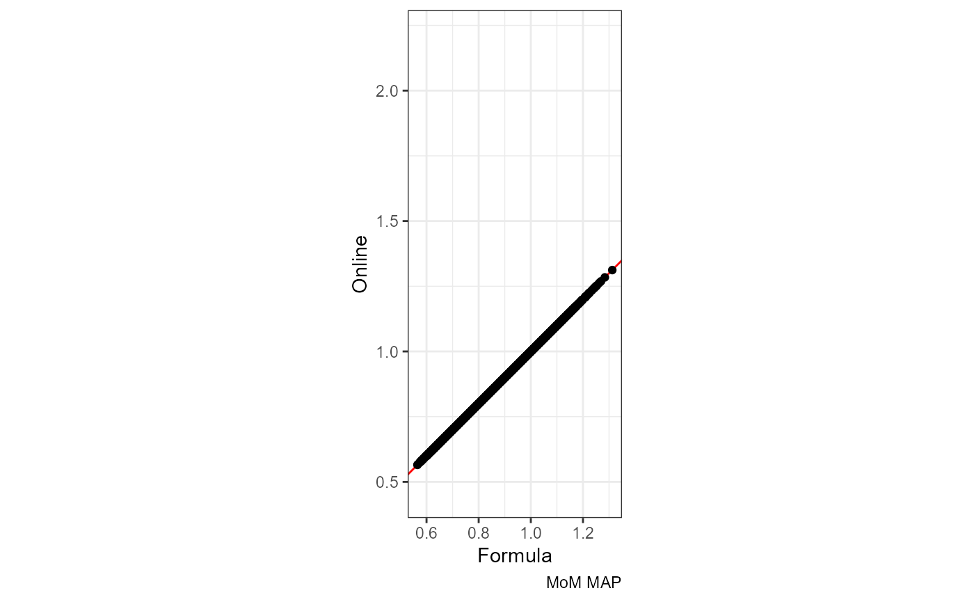
Mean vs Difference:
ggplot(df, aes((mom_MAP.x + mom_MAP.y) / 2, mom_MAP.y - mom_MAP.x)) +
    geom_point() +
  labs(x = "Mean", y = "Difference", caption = "MoM MAP")
#> Warning: Removed 318 rows containing missing values or values outside the scale range
#> (`geom_point()`).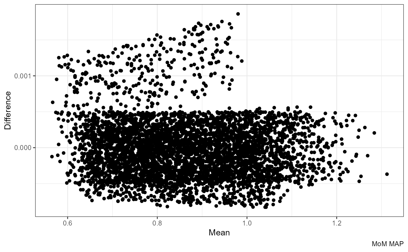
Difference:
ggplot(df, aes(mom_MAP.y - mom_MAP.x)) +
  geom_density() +
  labs(x = "Online - Formula", y = "Density", caption = "MoM MAP")
#> Warning: Removed 318 rows containing non-finite outside the scale range
#> (`stat_density()`).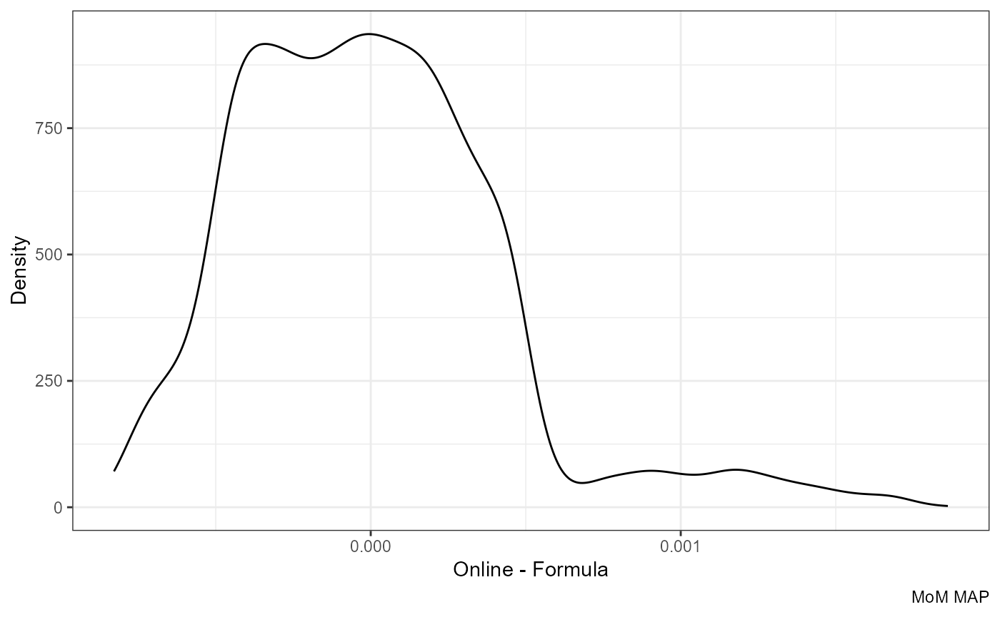
Note that the difference becomes even smaller if we round the formula-based values to three decimals:
ggplot(df, aes((round(mom_MAP.x, 3) + mom_MAP.y) / 2, mom_MAP.y - round(mom_MAP.x, 3))) +
    geom_point() +
  labs(x = "Mean", y = "Difference", caption = "MoM MAP")
#> Warning: Removed 318 rows containing missing values or values outside the scale range
#> (`geom_point()`).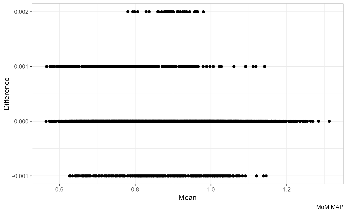
ggplot(df, aes(mom_MAP.y - round(mom_MAP.x, 3))) +
    geom_density() +
    labs(x = "Online - Formula", y = "Density", caption = "MoM MAP")
#> Warning: Removed 318 rows containing non-finite outside the scale range
#> (`stat_density()`).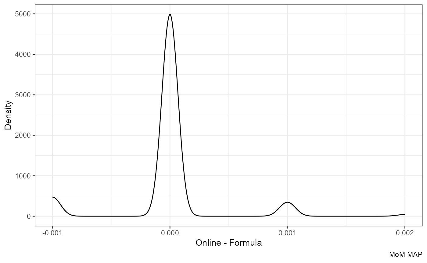
MoM UtAPI
The red line is x = y:
ggplot(df, aes(mom_PI.x, mom_PI.y)) +
  geom_abline(slope = 1, color = "red") +
  geom_point() + coord_equal() +
  labs(x = "Formula", y = "Online", caption = "MoM UtAPI")
#> Warning: Removed 672 rows containing missing values or values outside the scale range
#> (`geom_point()`).
Mean vs Difference:
ggplot(df, aes((mom_PI.x + mom_PI.y) / 2, mom_PI.y - mom_PI.x)) +
    geom_point() +
  labs(x = "Mean", y = "Difference", caption = "MoM UtAPI")
#> Warning: Removed 672 rows containing missing values or values outside the scale range
#> (`geom_point()`).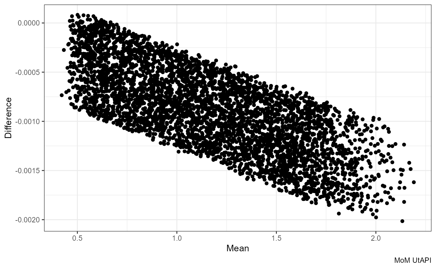
Difference:
ggplot(df, aes(mom_PI.y - mom_PI.x)) +
  geom_density() +
  labs(x = "Online - Formula", y = "Density", caption = "MoM UtAPI")
#> Warning: Removed 672 rows containing non-finite outside the scale range
#> (`stat_density()`).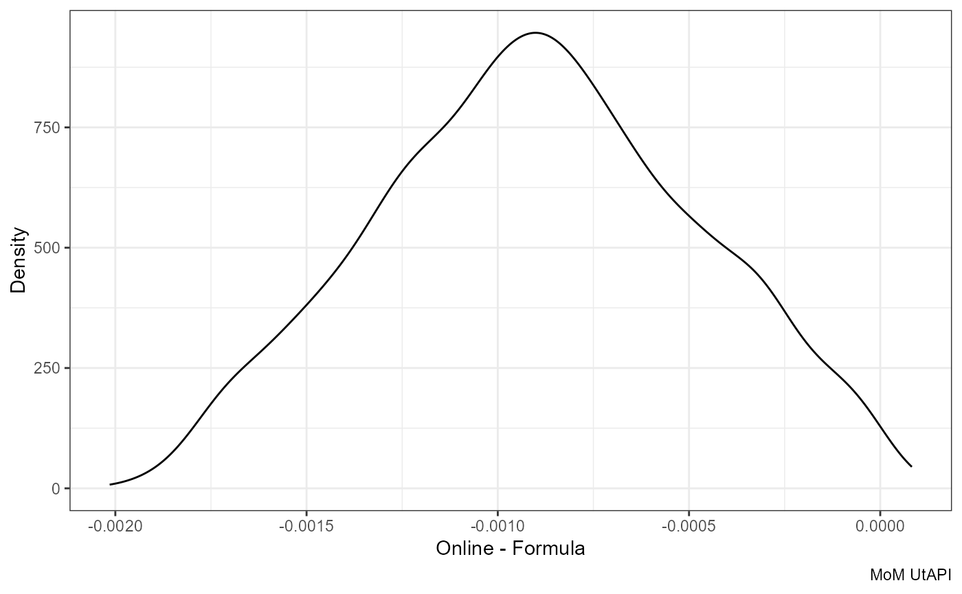
Round to three decimals:
ggplot(df, aes(mom_PI.y - round(mom_PI.x, 3))) +
  geom_density() +
  labs(x = "Online - Formula", y = "Density", caption = "MoM UtAPI")
#> Warning: Removed 672 rows containing non-finite outside the scale range
#> (`stat_density()`).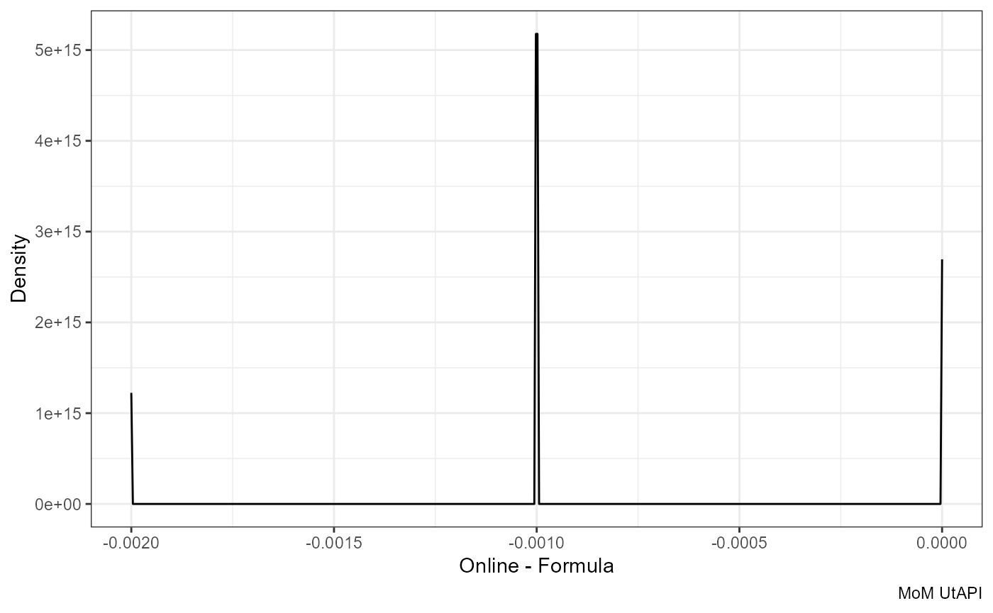
ggplot(df, aes((round(mom_PI.x, 3) + mom_PI.y) / 2, mom_PI.y - round(mom_PI.x, 3))) +
    geom_point() +
  labs(x = "Mean", y = "Difference", caption = "MoM UtAPI")
#> Warning: Removed 672 rows containing missing values or values outside the scale range
#> (`geom_point()`).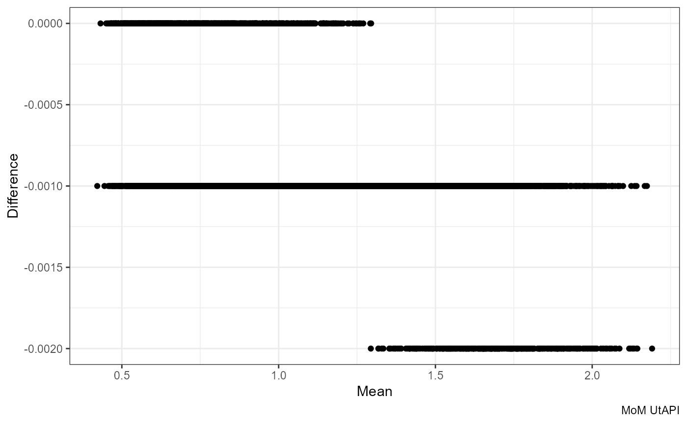
MoM PlGF
The red line is x = y:
ggplot(df, aes(mom_PlGF.x, mom_PlGF.y)) +
  geom_abline(slope = 1, color = "red") +
  geom_point() + coord_equal() +
  labs(x = "Formula", y = "Online", caption = "MoM PlGF")
#> Warning: Removed 334 rows containing missing values or values outside the scale range
#> (`geom_point()`).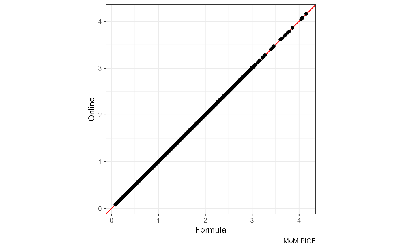
Mean vs Difference:
ggplot(df, aes((mom_PlGF.x + mom_PlGF.y) / 2, mom_PlGF.y - mom_PlGF.x)) +
    geom_point() +
  labs(x = "Mean", y = "Difference", caption = "MoM PlGF")
#> Warning: Removed 334 rows containing missing values or values outside the scale range
#> (`geom_point()`).
Difference:
ggplot(df, aes(mom_PlGF.y - mom_PlGF.x)) +
  geom_density() +
  labs(x = "Online - Formula", y = "Density", caption = "MoM PlGF")
#> Warning: Removed 334 rows containing non-finite outside the scale range
#> (`stat_density()`).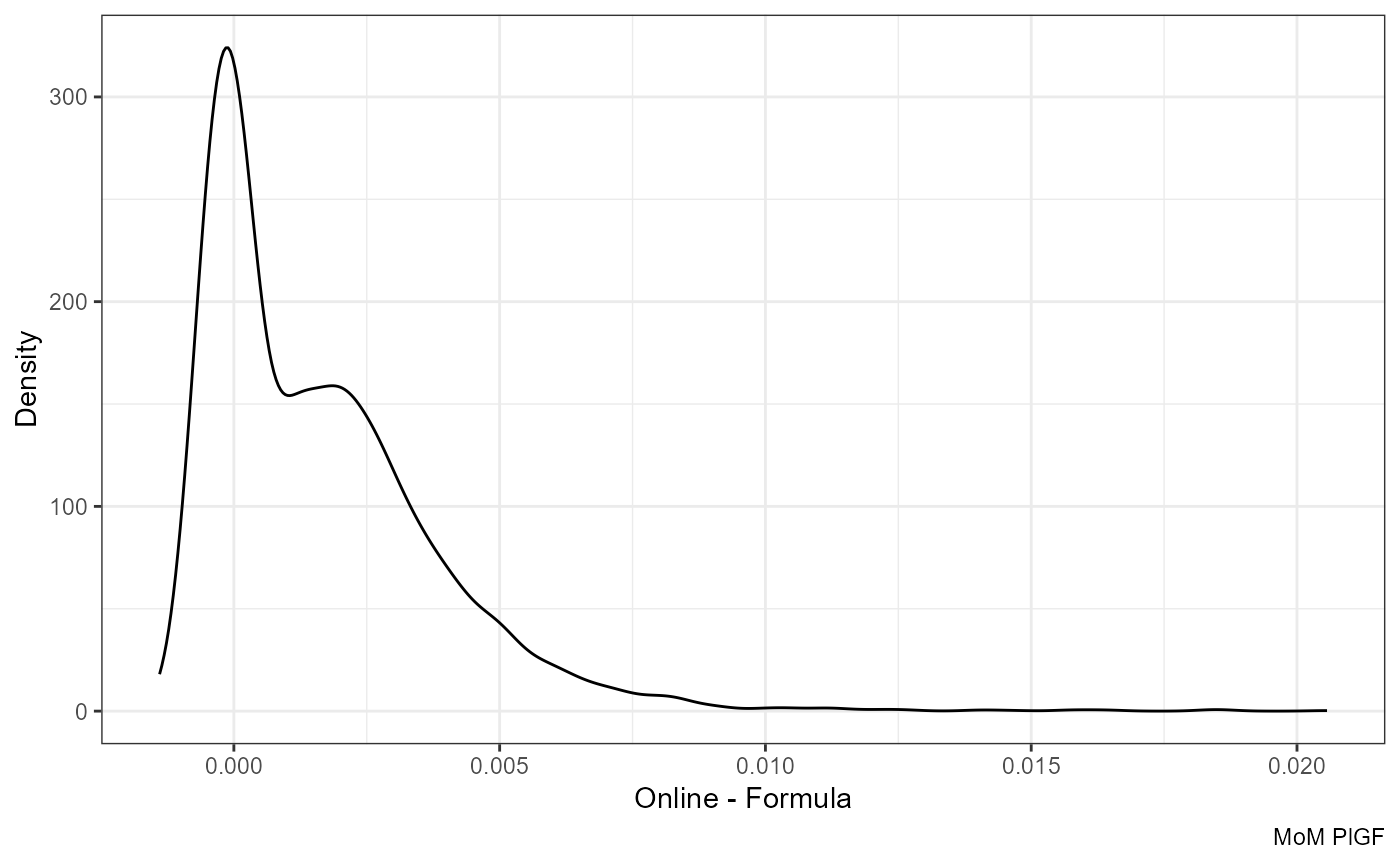
Prior risk
The red line is x = y:
ggplot(df, aes(nrisk_prior.x, nrisk_prior.y)) +
  geom_abline(slope = 1, color = "red") +
  geom_point() + coord_equal() +
  scale_x_log10() + scale_y_log10() +
  labs(x = "Formula", y = "Online", caption = "Prior risk")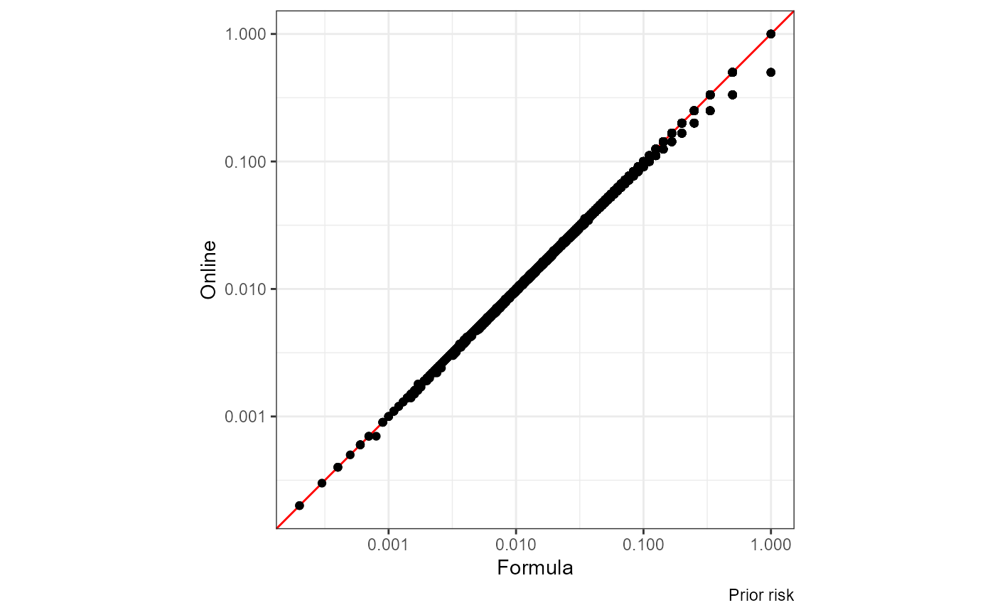
Mean vs Difference:
ggplot(df, aes((nrisk_prior.x + nrisk_prior.y) / 2, nrisk_prior.y - nrisk_prior.x)) +
    geom_point() + scale_x_log10() +
  labs(x = "Mean", y = "Difference", caption = "Prior risk")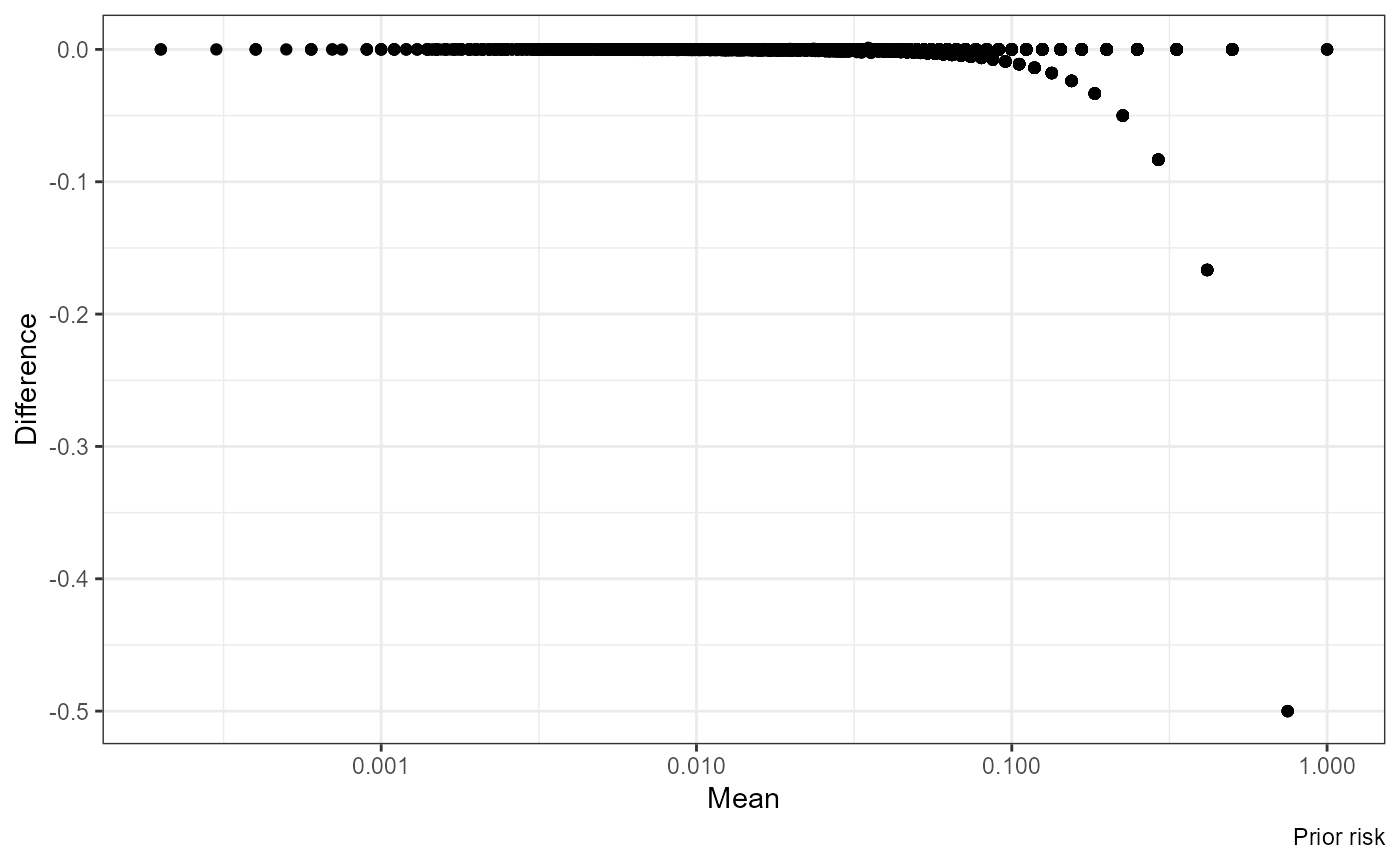
ggplot(df, aes((nrisk_prior.x + nrisk_prior.y) / 2, abs(nrisk_prior.y - nrisk_prior.x))) +
    geom_point() + scale_x_log10() + scale_y_log10() +
    labs(x = "Mean", y = "Abs. Difference", caption = "Prior risk")
#> Warning in scale_y_log10(): log-10 transformation introduced
#> infinite values.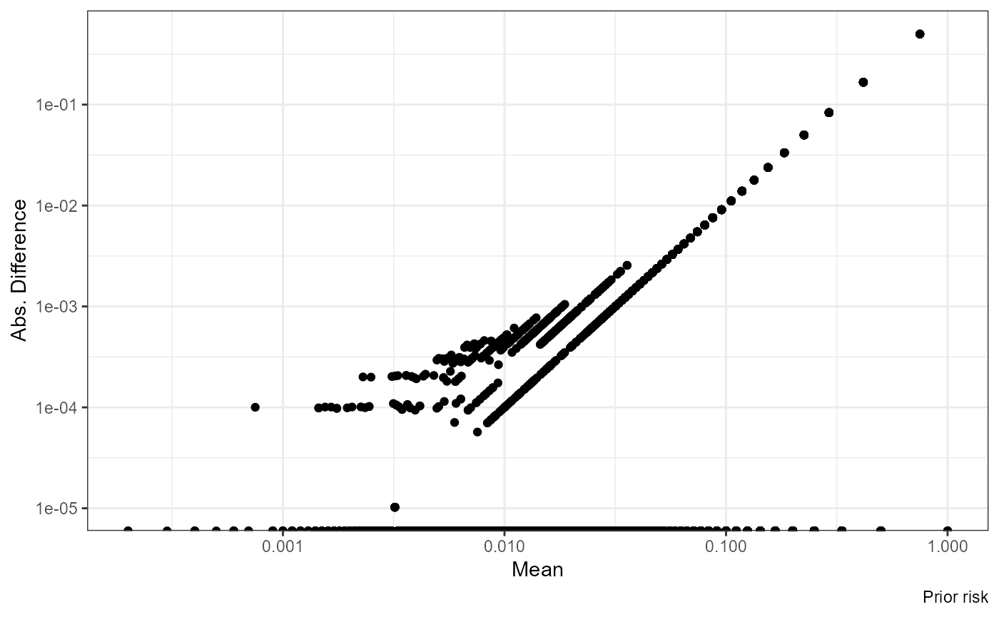
Difference:
ggplot(df, aes(nrisk_prior.y - nrisk_prior.x)) +
  geom_density() +
  labs(x = "Online - Formula", y = "Density", caption = "Prior risk")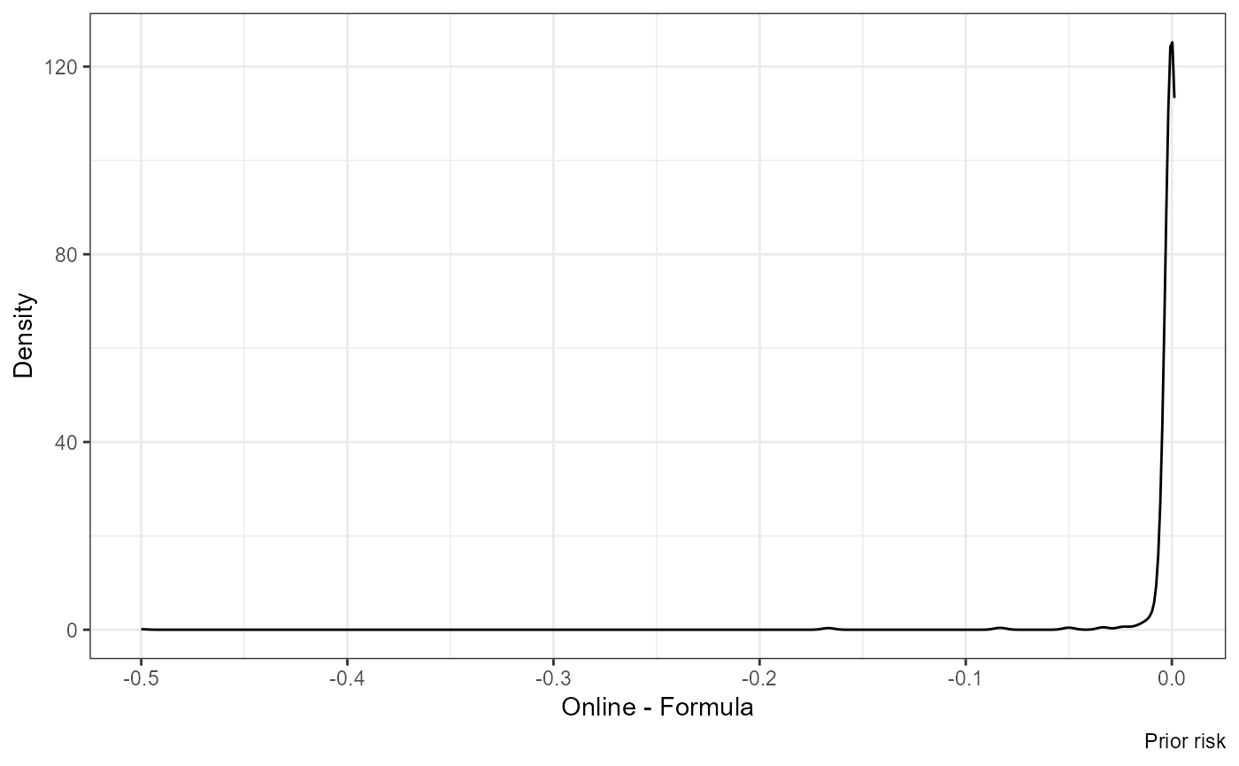
Risk score
The red line is x = y:
ggplot(df, aes(nrisk.x, nrisk.y)) +
  geom_abline(slope = 1, color = "red") +
  geom_point() + coord_equal() +
  scale_x_log10() + scale_y_log10() +
  labs(x = "Formula", y = "Online", caption = "Risk score")
#> Warning in scale_x_log10(): log-10 transformation introduced
#> infinite values.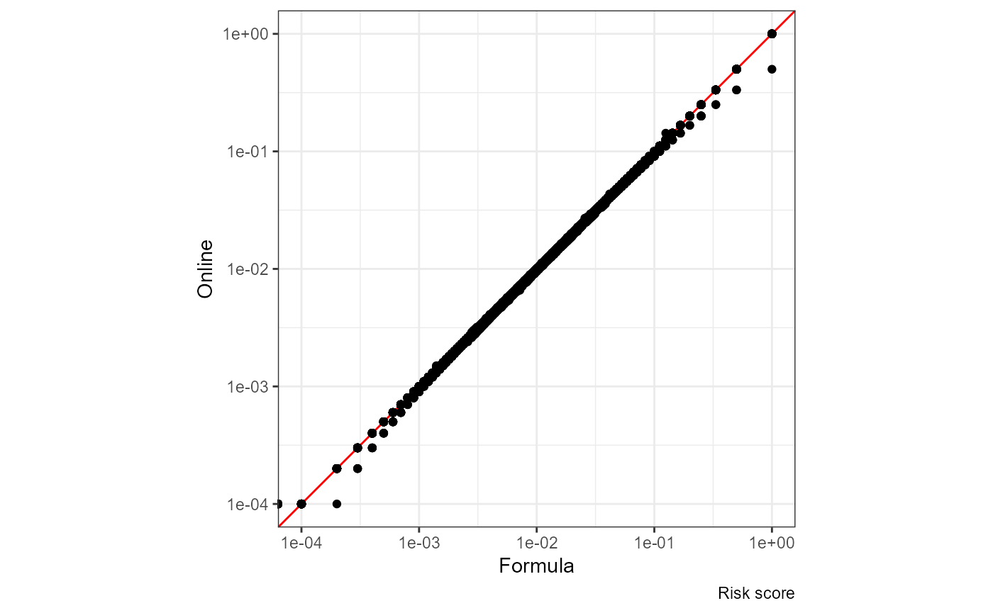
Mean vs Difference:
ggplot(df, aes((nrisk.x + nrisk.y) / 2, nrisk.y - nrisk.x)) +
    geom_point() + scale_x_log10() +
  labs(x = "Mean", y = "Difference", caption = "Risk score")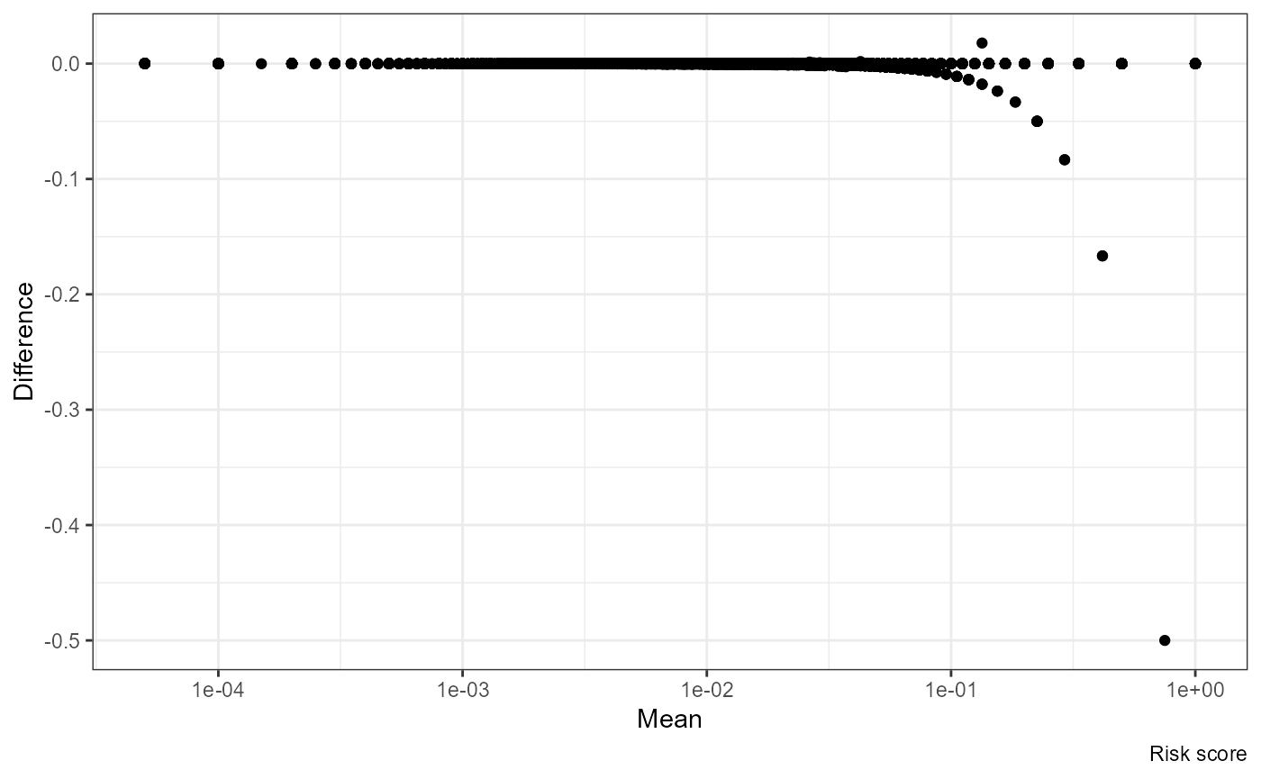
ggplot(df, aes((nrisk.x + nrisk.y) / 2, abs(nrisk.y - nrisk.x))) +
    geom_point() + scale_x_log10() + scale_y_log10() +
    labs(x = "Mean", y = "Abs. Difference", caption = "Risk score")
#> Warning in scale_y_log10(): log-10 transformation introduced
#> infinite values.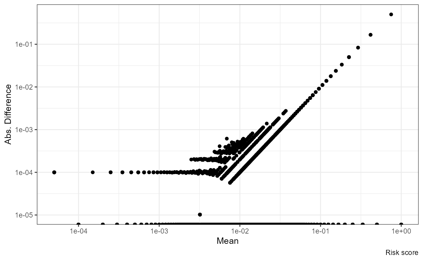
Difference:
ggplot(df, aes(nrisk.y - nrisk.x)) +
  geom_density() +
  labs(x = "Online - Formula", y = "Density", caption = "Risk score")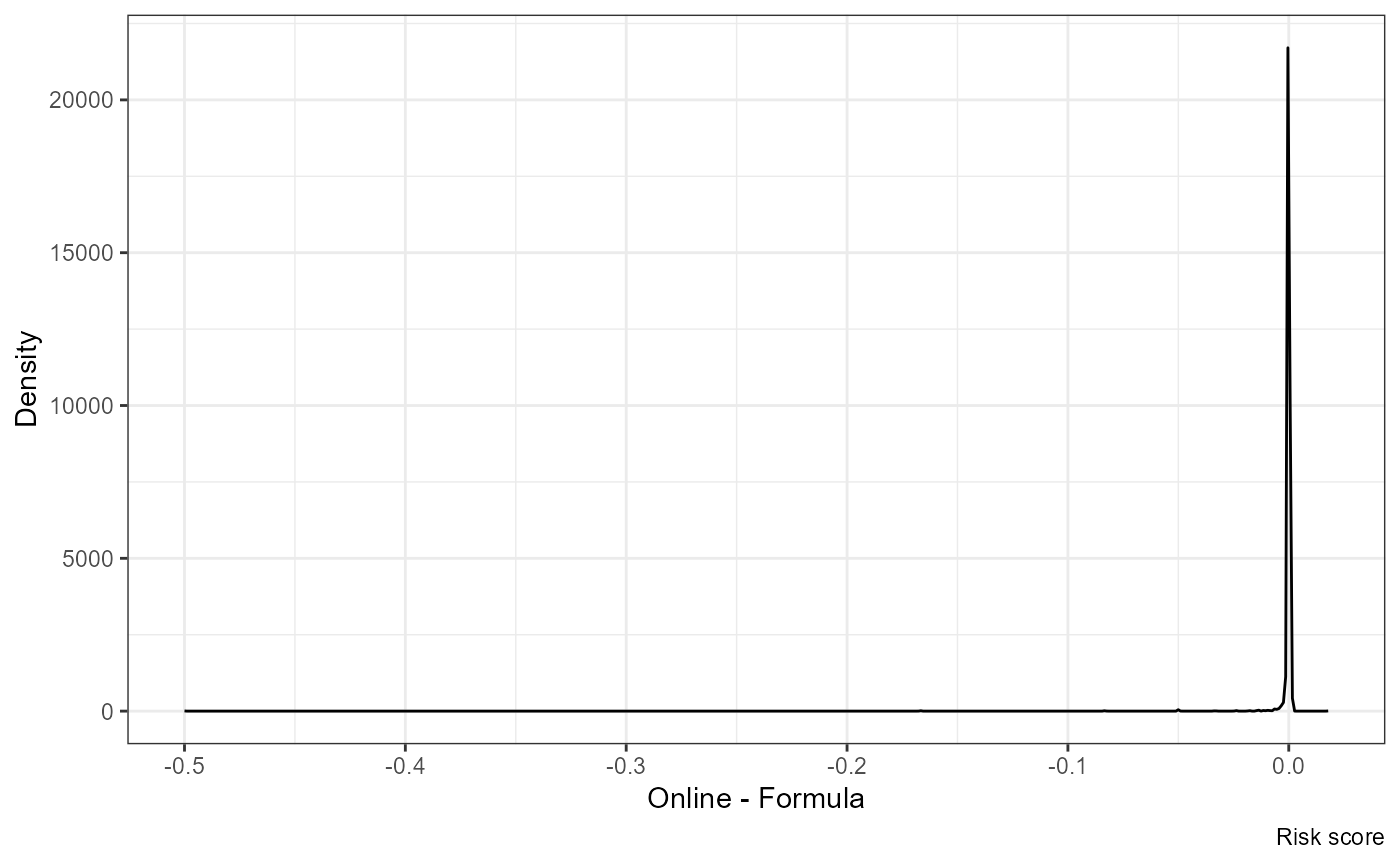
I guess some of this is related to rounding (it makes a big impact whether it is “1 in 3” vs “1 in 4”)
The most important thing, however, is related to the threshold of 1/100: