Introduction to ALASCA
The ALASCA package is described in the paper ALASCA: An R package for longitudinal and cross-sectional analysis of multivariate data by ASCA-based methods.. The paper contains several examples of how the package can be used.
This vignette will only show how to quickly get started with the ALASCA package. For more examples, see
Installation
if (!requireNamespace("devtools", quietly = TRUE))
    install.packages("devtools")

devtools::install_github("andjar/ALASCA", ref = "main")
Citation
If you have utilized the ALASCA package, please consider citing:
Jarmund AH, Madssen TS and Giskeødegård GF (2022) ALASCA: An R package for longitudinal and cross-sectional analysis of multivariate data by ASCA-based methods. Front. Mol. Biosci. 9:962431. doi: 10.3389/fmolb.2022.962431
@ARTICLE{10.3389/fmolb.2022.962431,
  AUTHOR={Jarmund, Anders Hagen and Madssen, Torfinn Støve and Giskeødegård, Guro F.},
  TITLE={ALASCA: An R package for longitudinal and cross-sectional analysis of multivariate data by ASCA-based methods},
  JOURNAL={Frontiers in Molecular Biosciences},
  VOLUME={9},
  YEAR={2022},
  URL={https://www.frontiersin.org/articles/10.3389/fmolb.2022.962431},
  DOI={10.3389/fmolb.2022.962431},
  ISSN={2296-889X}
}
Creating an ASCA model
Generating a data set
We will start by creating an artificial data set with 100 participants, 5 time points, and 20 variables. The variables follow four patterns
- Linear increase
- Linear decrease
- A v-shape
- An inverted v-shape
n_time     <- 5
n_id       <- 100
n_variable <- 20

df <- rbindlist(lapply(seq(1,n_id), function(i_id) {
  rbindlist(lapply(seq(1,n_variable), function(i_variable) {

    r_intercept <- rnorm(1, sd = 5)
    beta <- 2 + rnorm(1)

    temp_data <- data.table(
                  id = paste0("id_", i_id),
                  time = seq(1, n_time) - 1,
                  variable = paste0("variable_", i_variable)
                )
    if ((i_variable %% 4) == 0) {
      temp_data[, value := r_intercept + beta * time]
    } else if ((i_variable %% 4) == 1) {
      temp_data[, value := r_intercept - beta * time]
    } else if ((i_variable %% 4) == 2) {
      temp_data[, value := r_intercept - beta*n_time/2 + beta * abs(time - n_time/2)]
    } else {
      temp_data[, value := r_intercept + beta*n_time/2 - beta * abs(time - n_time/2)]
    }

    temp_data[, value := value + rnorm(n_time)]
    temp_data[, value := value * i_variable/2]
    temp_data
  }))
}))
Overall (ignoring the random effects), the four patterns look like this:
ggplot(df[variable %in% c("variable_1", "variable_2", "variable_3", "variable_4"),],
       aes(time, value)) +
  geom_smooth() +
  facet_wrap(~variable, scales = "free_y") +
  scale_color_viridis_d(end = 0.8)
#> `geom_smooth()` using method = 'loess' and formula = 'y ~ x'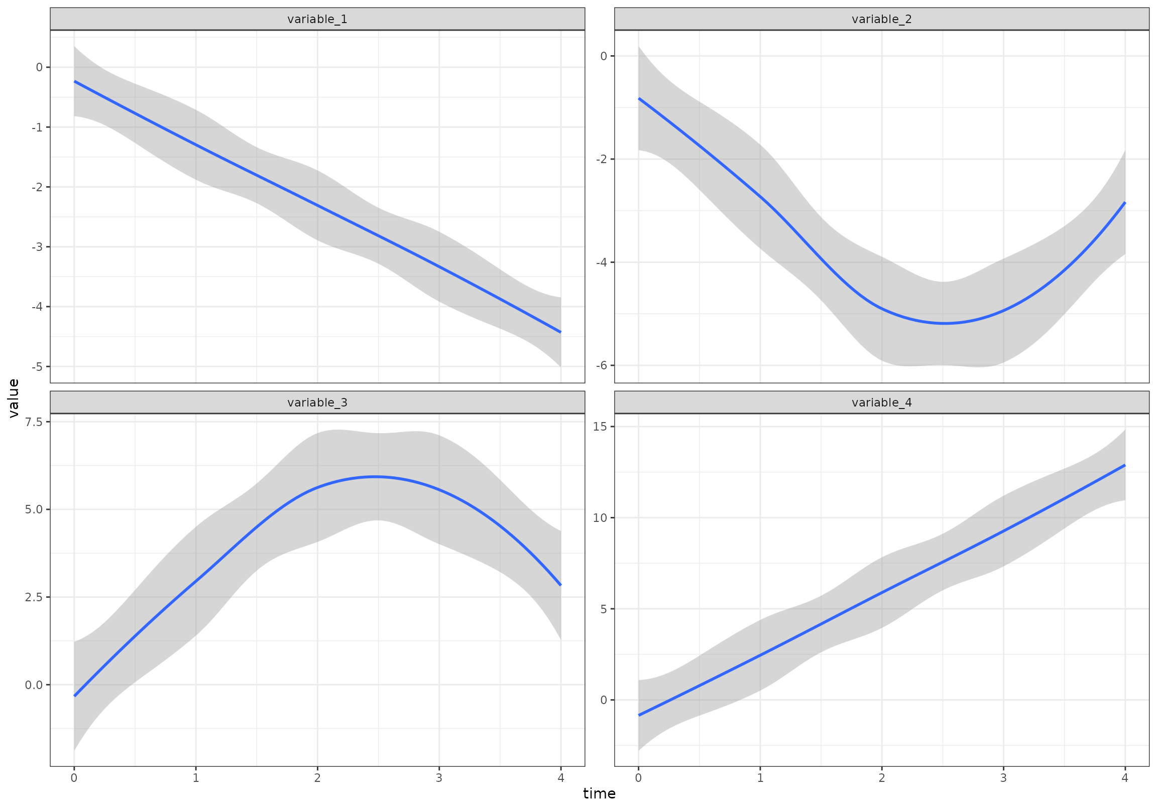
Data format
We want time to be a categorical variable:
df[, time := paste0("t_", time)]Your data can either be provided in long or wide format. In long format, there is one column with variable names and one column with the variable values. For example:
head(df)
#>        id   time   variable     value
#>    <char> <char>     <char>     <num>
#> 1:   id_1    t_0 variable_1 -4.718741
#> 2:   id_1    t_1 variable_1 -4.630553
#> 3:   id_1    t_2 variable_1 -5.444649
#> 4:   id_1    t_3 variable_1 -6.308879
#> 5:   id_1    t_4 variable_1 -8.921652
#> 6:   id_1    t_0 variable_2 -1.519332
In wide format, each variable has a separate column:
head(dcast(data = df, ... ~ variable))
#> Key: <id, time>
#>        id   time variable_1 variable_10 variable_11 variable_12 variable_13
#>    <char> <char>      <num>       <num>       <num>       <num>       <num>
#> 1:   id_1    t_0 -4.7187406  -11.026663  -33.089986   -3.840034   -34.79853
#> 2:   id_1    t_1 -4.6305530   -4.934307  -26.580592   21.281080   -39.04885
#> 3:   id_1    t_2 -5.4446495  -13.713424   -8.068981   30.558467   -55.43503
#> 4:   id_1    t_3 -6.3088786  -11.928633  -12.438091   40.293948   -80.95647
#> 5:   id_1    t_4 -8.9216517  -18.756847  -24.545307   52.171637   -95.93505
#> 6:  id_10    t_0 -0.7859144  -18.894901   33.717402  -28.553972   -12.28457
#>    variable_14 variable_15 variable_16 variable_17 variable_18 variable_19
#>          <num>       <num>       <num>       <num>       <num>       <num>
#> 1:   36.941850   46.476887  -31.914822    15.82093    52.32281   23.653014
#> 2:   19.270624   56.265443  -14.272835    15.82136    24.44972   47.001762
#> 3:    6.236771   67.005861    3.269452   -11.89028   -20.59183   50.792265
#> 4:   -7.953935   68.964827    5.302415   -43.06267   -23.46267   69.719916
#> 5:   22.492017   48.984122    7.309857   -39.87107    12.12405   45.952679
#> 6:    8.417839   -1.126344   51.693367    27.96056    36.83526   -9.563653
#>    variable_2 variable_20 variable_3 variable_4 variable_5 variable_6
#>         <num>       <num>      <num>      <num>      <num>      <num>
#> 1: -1.5193320   -60.71243   3.060183   5.105065  -7.996454 -2.8476669
#> 2: -3.5461263   -63.25700   3.969782   8.797435 -11.112641 -3.2200307
#> 3: -4.1192453   -47.02304   5.068662   6.216448 -12.163650  0.6524932
#> 4: -2.6832024   -24.65360   2.883055   5.930557  -9.932992 -2.3393258
#> 5: -4.6234163   -22.37929   4.750917   9.161264 -14.930770 -4.1970628
#> 6: -0.4602348    41.75252  -6.688525   5.760711   4.077213  1.5739838
#>    variable_7 variable_8 variable_9
#>         <num>      <num>      <num>
#> 1:  0.6824042 -39.207357  -52.79308
#> 2: 14.8893837 -27.610413  -71.27899
#> 3: 11.5280900 -15.261008  -88.47604
#> 4: 13.3872119  -3.771129 -117.37500
#> 5:  5.6591043   9.758284 -130.44083
#> 6:  6.1093436 -25.185080  -28.99145
ALASCA supports both formats but defaults to long format. To use wide
format, you have to set wide = TRUE.
Initialize an ALASCA model
In this example, we are only looking at the common time development. For examples involving group differences, see the vignette on regression models.
To assess the time development in this data set, we will use the
regression formula value ~ time + (1|id). Here,
value is the measured variable value, time the
predictor, and (1|id) a random intercept per
participant-id. ALASCA will implicitly run the regression for each
variable separately.
res <- ALASCA(
  df,
  value ~ time + (1|id)
)
#> INFO  [2026-03-14 17:20:13] Initializing ALASCA (v1.0.20, 2026-03-14)
#> WARN  [2026-03-14 17:20:13] Guessing effects: `time`
#> INFO  [2026-03-14 17:20:13] Will use linear mixed models!
#> INFO  [2026-03-14 17:20:13] Will use Rfast!
#> WARN  [2026-03-14 17:20:13] The `time` column is used for stratification
#> WARN  [2026-03-14 17:20:13] Converting `character` columns to factors
#> INFO  [2026-03-14 17:20:13] Scaling data with sdall ...
#> INFO  [2026-03-14 17:20:13] Calculating LMM coefficients
#> INFO  [2026-03-14 17:20:13] ==== ALASCA has finished ====
#> INFO  [2026-03-14 17:20:13] To visualize the model, try `plot(<object>, effect = 1, component = 1, type = 'effect')`
The ALASCA function will provide output with important information:
-
Guessing effects: 'time'When effects are not explicitly provided to ALASCA, the package will try to guess the effects you are interested in. See the vignette on regression models for details. -
Will use linear mixed models!ALASCA will use linear mixed models when you provide a random effect in the regression formula (i.e.,(1|id)) -
Will use Rfast!Linear mixed model regression can be performed by one out of two different R packages: the lme4 package or the Rfast package -
The 'time' column is used for stratificationThis is only important for model validation. For details, see the vignette on model validation -
Converting 'character' columns to factorsWe provided time as a character variable and ALASCA converts it to a factor variable. If the levels of your variable matters and they are not in alphabetical order, you may want to convert the variable to a factor by yourself. -
Scaling data with sdall ...ALASCA supports various scalings, andsdallis the default. For details, see our paper ALASCA: An R package for longitudinal and cross-sectional analysis of multivariate data by ASCA-based methods. -
Calculating LMM coefficientsSimply informs you that the regression is ongoing as this may take some time
To see the resulting model:
plot(res, component = c(1,2), type = 'effect')
#> INFO  [2026-03-14 17:20:13] Effect plot. Selected effect (nr 1): `time`. Component: 1 and 2.
See the vignette on plotting the model for more visualizations.